This example shows the basics of how to use a filter in GNU Radio. First, we have to generate a set of filter taps, which can be a vector of either real complex values. While you are welcome to generate the taps any way you would like, GNU Radio provides a few generating functions to make this easier.

Basic Filters

The first example shows the use of the "firdes" utility, which is used to generate windowed FIR filters. Here, I am creating a simple low pass filter (LPF). There are generally two versions of each type of filter. Those with the "_2" extension provide a means of specifying the out-of-band (or stopband) attenuation (in dB). Generally, you want to use this version as it costs you almost nothing but gives you an extra parameter to control.

Example code: filter_basics.py

In this example, we create a low pass filter using the function:

lpf_taps = filter.firdes.low_pass_2(1, 1, 0.2, 0.1, 60)

We are specifying, in order, the filter gain, sample rate, center of the transition band, the transition band width, and the stopband attenuation (in dB). The center of the transition band specifies the point where the rolloff is 6 dB down from the passband. This value and the transition band are set relative to the sample rate. Since the sample rate here is set to 1.0, we must also specify normalized bandwidths. We can also use a real sample rate here and scale the widths appropriately in terms of Hz.

The filter_basics.py example shows the use of two filters: filter.fir_filter_ccc and filter.fft_filter_ccc. These take the same arguments and both filter a signal with the same filter taps. The difference is in how they do it. The version with "fir_" performs a straight-forward implementation of an FIR filter by performing the convolution in time. The "fft_" version, however, performs the fast-convolution, which means that it takes an FFT and performs the convolution as a multiplication in the frequency domain. The results are then passed through an IFFT to get the samples back into the time domain.

For small filters, which is somewhere around 30-taps and fewer, the FIR filter version performs faster. However, the fast-convolution takes advantage of faster multiplies and the inexpensive FFT and IFFT operations. For larger filters (greater than 30), these operations perform better than the FIR filter.

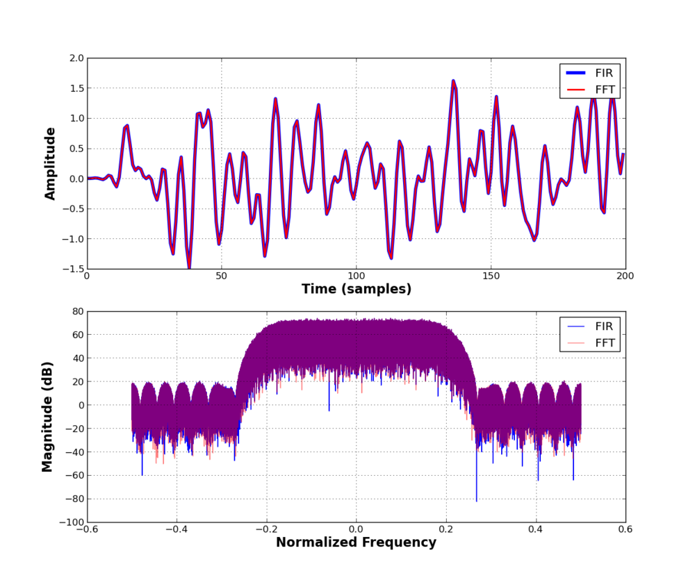
The figure below shows the output of filtering a noise signal with both an FIR and FFT version of the same filter. While this does not show off the difference in speed, it shows that the output is the same. In time, they look almost identical. In the frequency domain, we can see a slight difference due to numerical precision that is negligable.

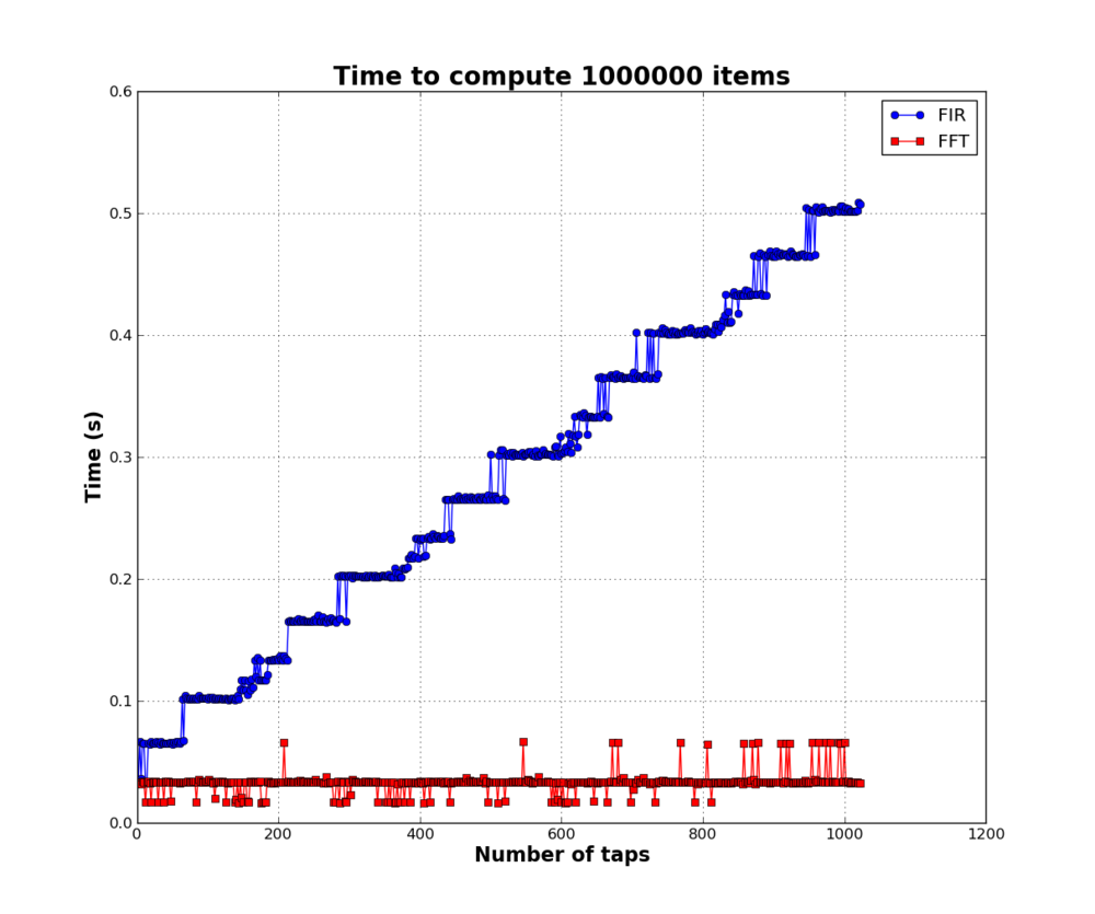
To compare the processing time of the different filers, you can use the filter_timing.py file. It takes a few minutes to run as is. The variables N, start, stop, and step can be easily changed to examine different aspects of the behavior. Looking at the times for 1024 taps (sampled every 2 taps) produces the following image. This was on an Intel i7-2620M CPU with AVX enabled in VOLK. The FIR filter climbs nearly linearly, though the step-wise pattern is likely related to something in the VOLK vectorized processing. However, the FFT filter is nearly flat over all filter sizes. It also shows that on this processor, the crossover point is a very small number of taps; in fact, it's close to 1.

Windowed and Parks-McClellen Filters

The second example shows the use of a second GNU Radio filter design utility called "optfir" module, also a part of the "filter" module. However, the optfir module is built entirely in Python while firdes is written in C++. This filter designer uses the Parks-McClellen algorithm for designing filters. Unlike the firdes windowed filters, this utility gives you another degree of freedom when designing filters: the passband ripple (in dB).

You have to watch out for this utility, though, especially if you are comfortable with using firdes. In the firdes utility, you specify the center of the transition band, which is 0.5 in linear amplitude or -6 dB in log power scale. You also specify the transition band, which is the width from the cutoff to the stopband. On the other hand, in the optfir utility, you will specify the end of the passband(s) and start of the stopband(s) (plural if you are designing bandpass filters). The end of the passband is the point when the filter roll-off begins, not the 3-dB or 6-dB point, and the start of the stopband is where the first null occurs. Keep in mind, though, that these values are going to be approximate since the Parks-McClellen algorithm is an optimization technique that attempts to fit a filter to the desired specs.

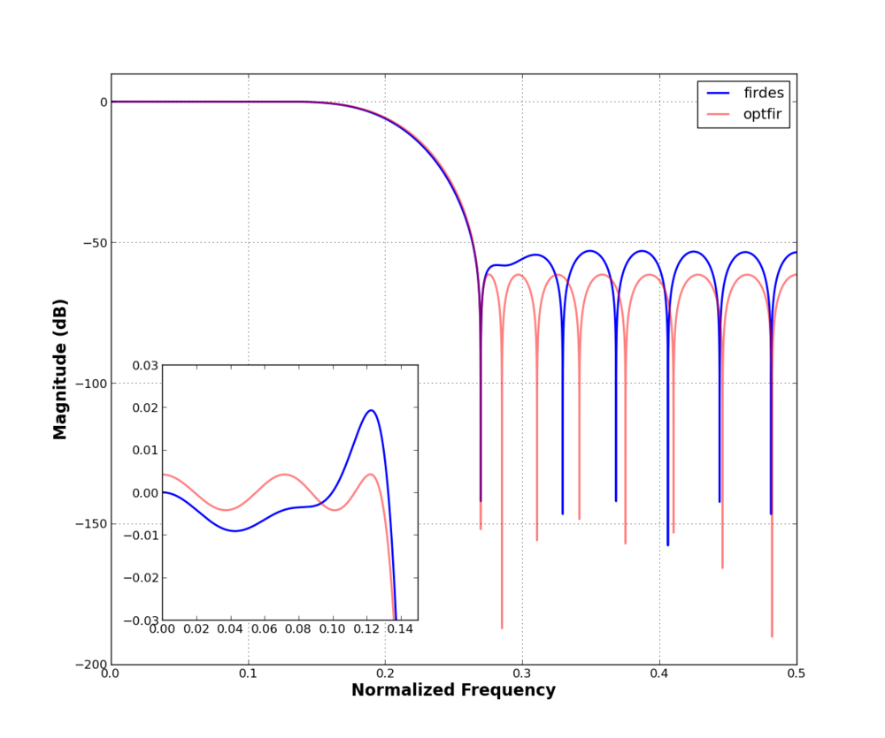
In the following example, I tried to design a LPF with both the firdes and optfir filters that were approximately the same filter, by which I mean having the same passband and stopband. What is different is that the specified passband ripple from optfir gives me a much lower ripple for the same number of filter taps (27 in this case). If we specified a ripple of, say 0.03 dB, we can reduce the filter size a bit farther. The point here being that for approximately equivalent filters, you are generally going to get a smaller filter using the Parks-McClellen.

We create the taps with the following function calls.

firdes_taps = filter.firdes.low_pass_2(1, 1, 0.2, 0.1, 60)

optfir_taps = filter.optfir.low_pass(1, 1, 0.13, 0.2675, 0.01, 60)

Filter example with optfir: filter_optfir.py